VI Phenology
Per-pixel datacubes, 19 phenological metric maps and model-ready rasters from vegetation index time series.
The companion to the HLS Vegetation Index Pipeline. It reads any CF-1.8 NetCDF with time × y × x dimensions and turns raw, irregularly sampled vegetation index observations into phenology science products.
Four pipelines
| Pipeline | Produces |
|---|---|
netcdf_datacube |
Per-pixel CF-1.8 datacubes clipped to study polygons. This is the foundation for everything else. |
phenology |
ROI-mean time series, smoothing, phenological metrics, and PNG + interactive HTML plots |
pixel_phenology |
19 per-pixel metric maps: peak, productivity, seasonality, variability, bimodality |
datacube_to_geotiff |
Per-year, per-month and per-day-of-year statistics as multi-band GeoTIFFs for downstream models |
Science choices
- Smoothing: Savitzky-Golay, LOESS, harmonic, linear or Whittaker. Whittaker handles HLS’s irregular revisit cadence without binning.
- Metrics: start, peak and end of season, season length, integrated VI, green-up and senescence rates, plus extended metrics (floor/ceiling NDVI, bimodality, coefficient of variation) taken directly from the smoothed curve, so no biome-specific day-of-year windows are needed.
- Robust sampling: fixed per-region pixel samples, NDVI and quality filters, and minimum-observation thresholds keep cloud masking and sparse years from biasing the metrics.
Scale
Per-pixel work runs in parallel with a sparse SciPy solver that releases Python’s GIL. GeoTIFF output is written band by band, so peak memory is one spatial band no matter how large the output is. The per-day-of-year product alone holds 1,095 bands.
Where it’s used
NASA BioSCape: VI Phenology builds the CF-1.8 NetCDF datacubes of time-series phenology that I delivered for this NASA-funded project in South Africa, which were used as model inputs for the project. The BioSCape Phenology Explorer lets researchers explore them.
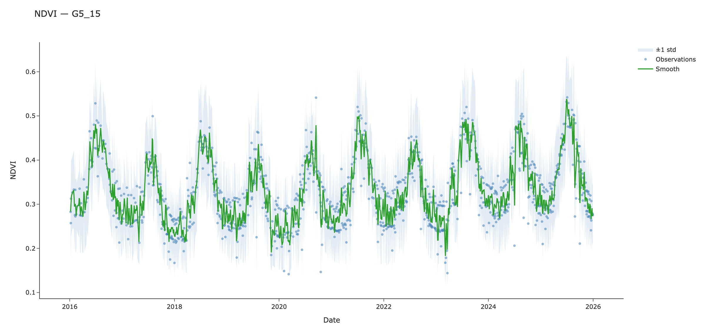
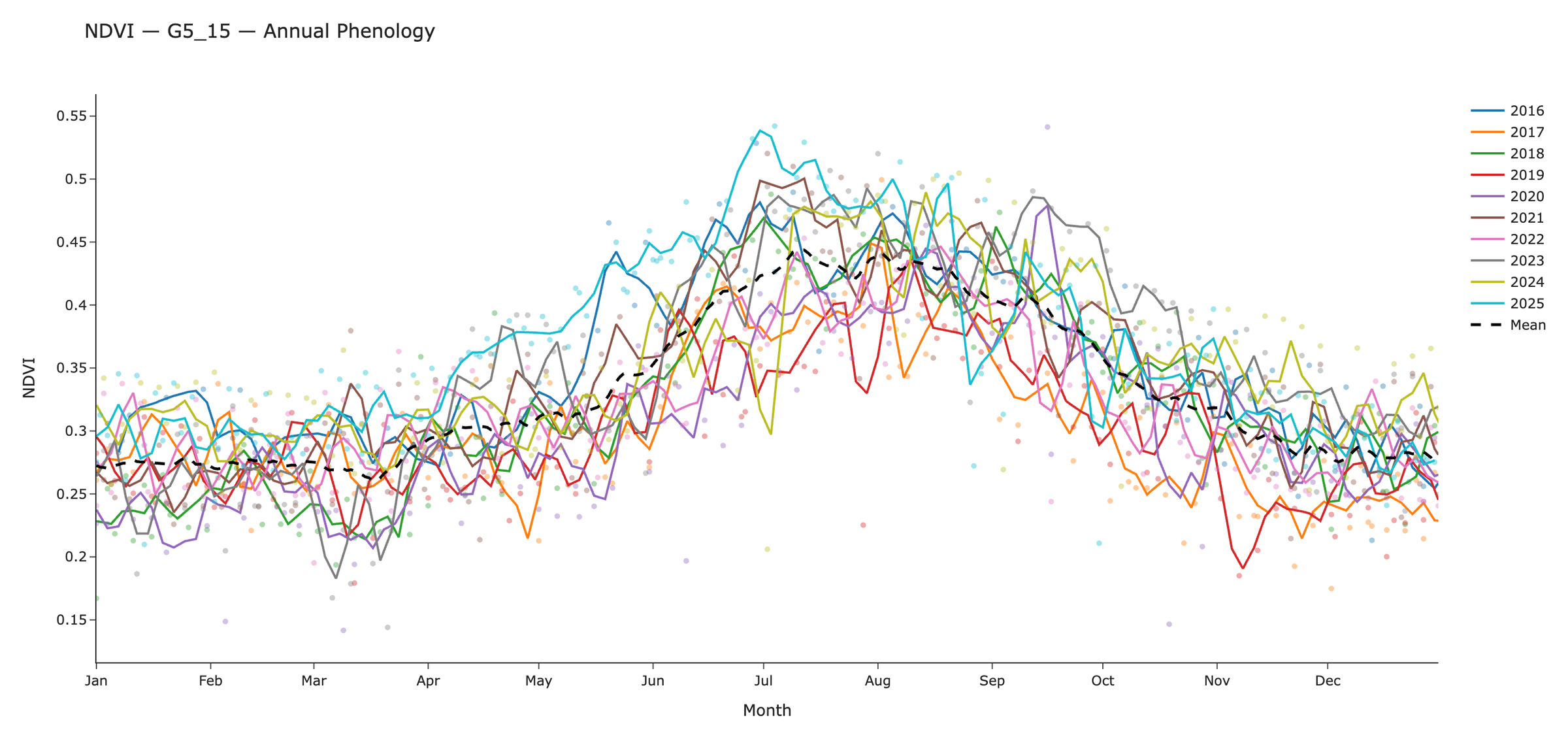
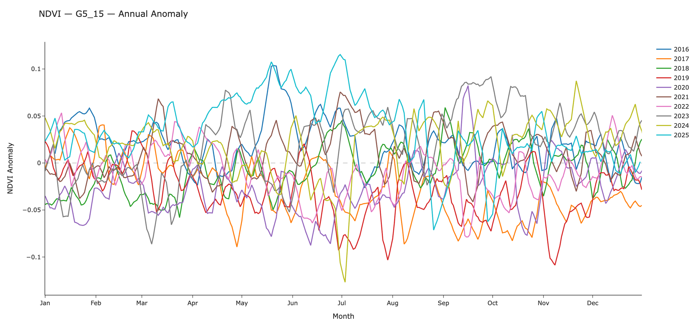
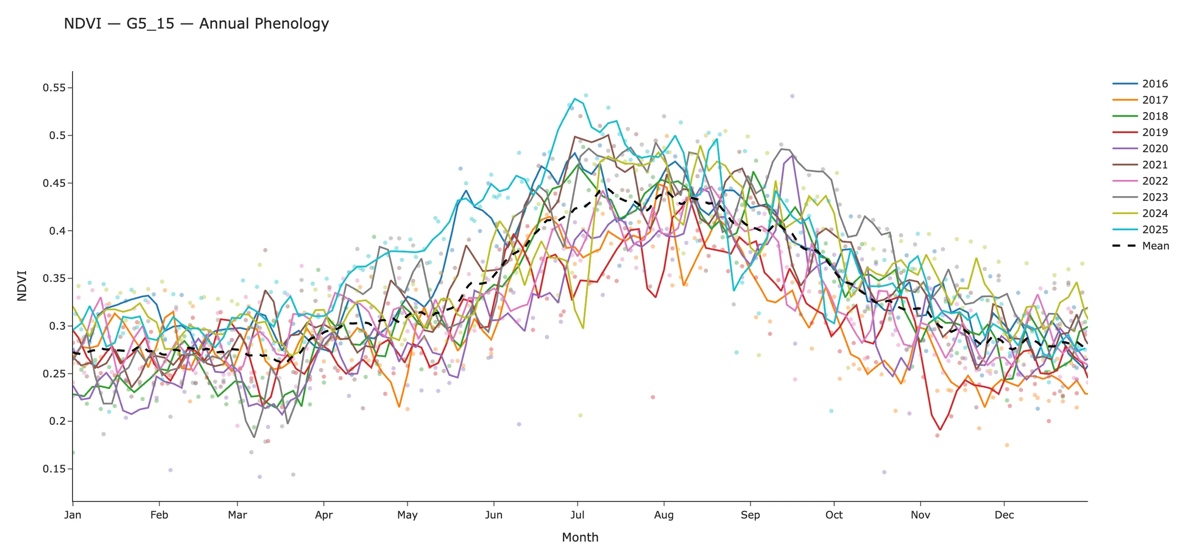
Phenology plots: one BioSCape flight box
Outputs of the phenology pipeline for LVIS flight box G5_15 in South Africa’s Cape, 2016–2025. Each plot is also produced as an interactive HTML version.